[solved] Converting angular displacement to HPR for a billiard ball (gif inside)

[ekiefl]

Hi everyone,

I’m making a physics pool engine in python and cannot seem to get the ‘roll’ of the balls to work. In my application, the ball histories are all precomputed. So I basically have an array that stores, as a function of time, the

1. linear velocity
2. displacement vector
3. angular velocity of each ball around its center of mass
4. the “angular displacement”, i.e. the time integration of angular velocity

I’ve had a lot of success so far translating the balls with panda3d, but giving them the correct roll using the angular displacement has been extremely difficult. What I’m currently doing to calculate Heading Pitch Roll (HPR) from angular displacement is this:

I have an array of angular displacements, which is like the integral of angular velocity. So for example, if a ball spins with an angular velocity <0,0,1> for 2 seconds, the angular displacement would be <0,0,2>. To convert this into HPR, I am using scipy:

import numpy as np
from scipy.spatial.transform import Rotation

def as_euler_angle(theta):
    return Rotation.from_rotvec(theta).as_euler('zxy', degrees=True)

print(as_euler_angle(np.array([0,0,2])))

This yields [114.5915590262 0. 0. ], i.e. it changes the Heading, as expected.

As a reminder, I have this precomputed for each timepoint, and so to update the positions and orientations of the ball I have an update method I call each frame:

    def update(self, frame):
        self.node.setPos(self.xs[frame], self.ys[frame], self.zs[frame] + self._ball.R)
        self.node.setHpr(self.hs[frame], self.ps[frame], self.rs[frame])

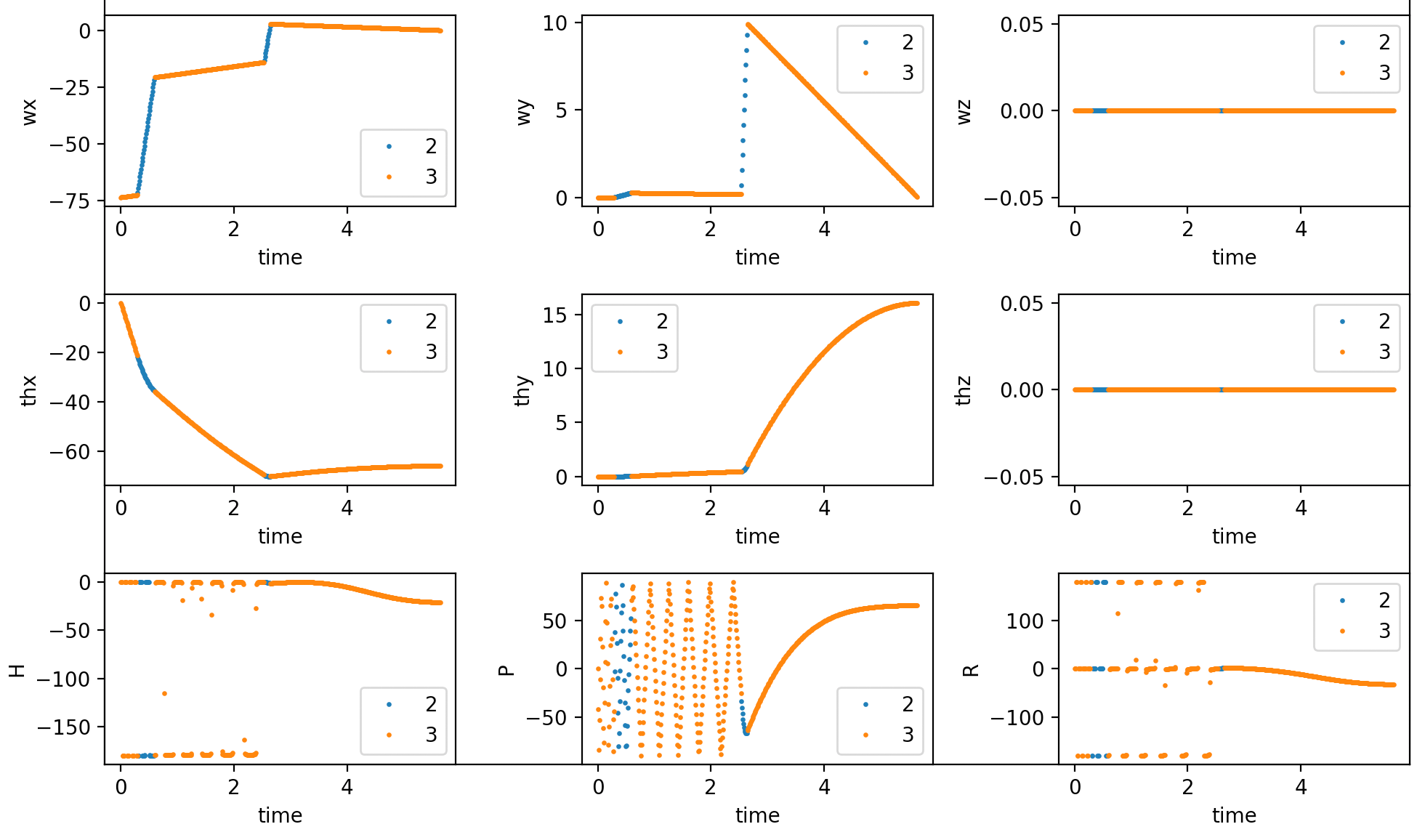
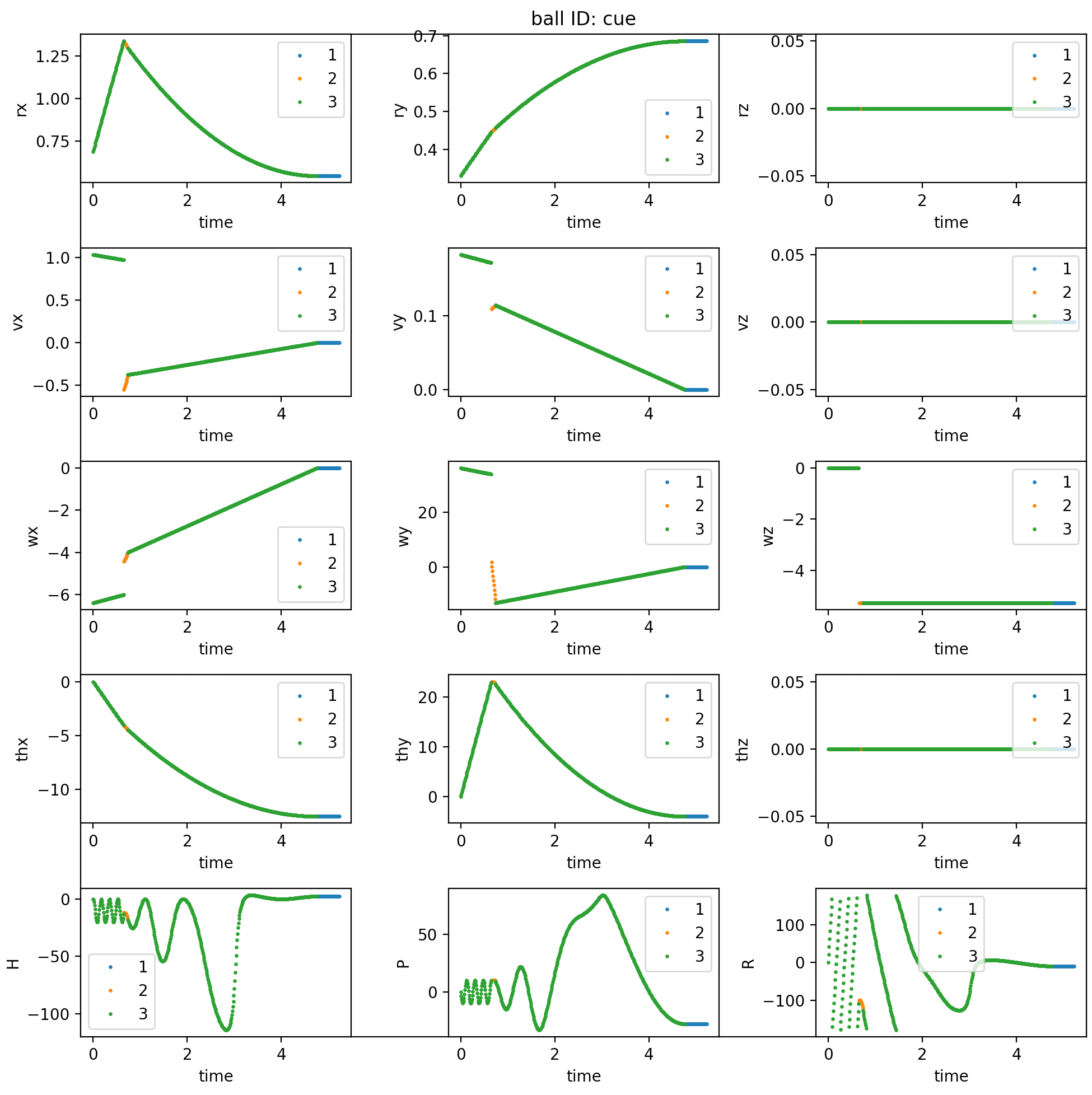
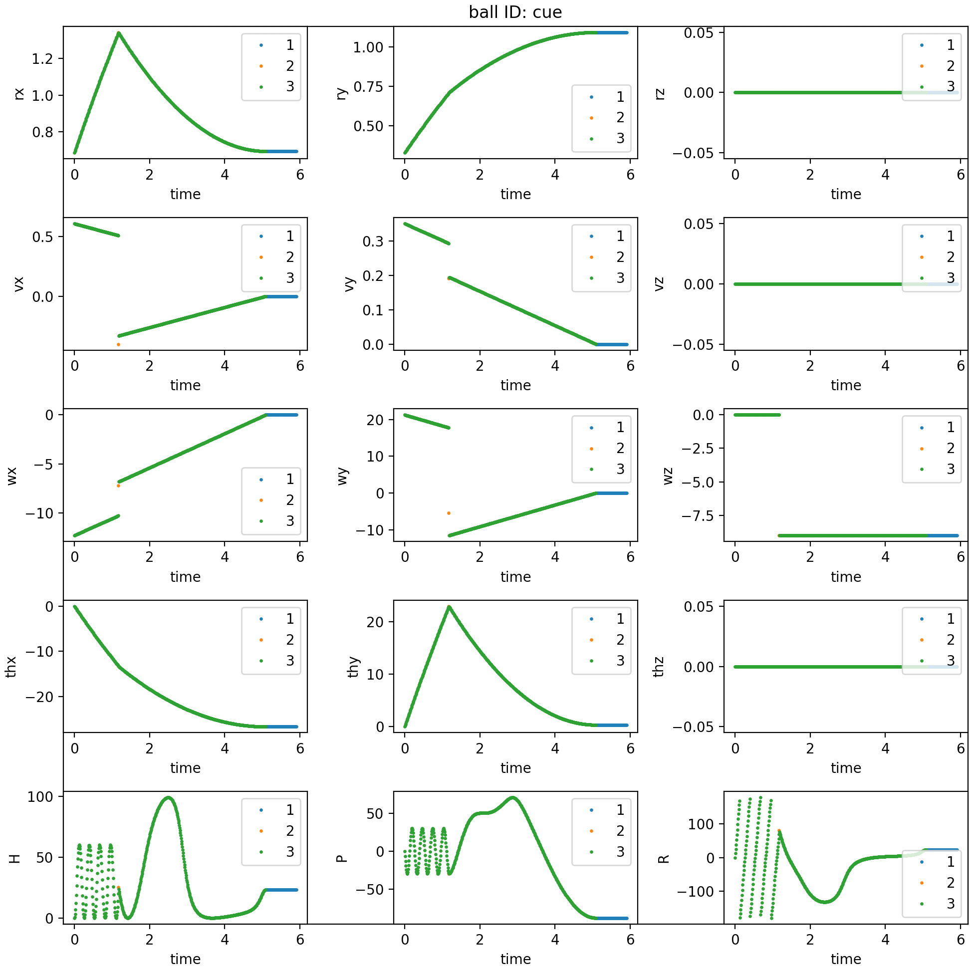
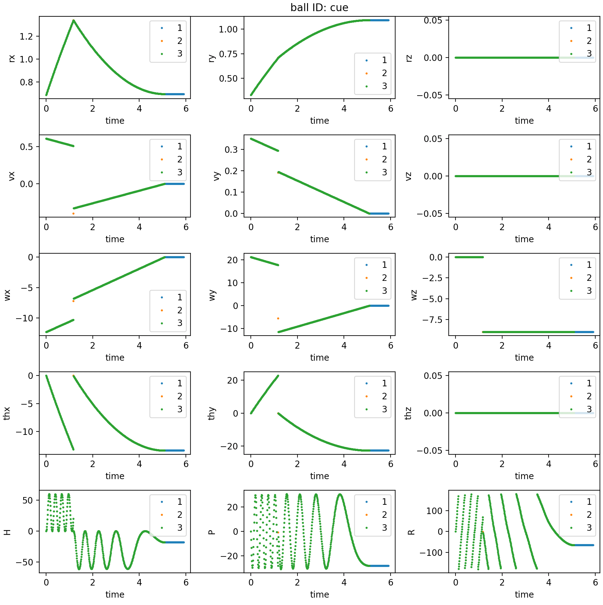
This works perfectly for translating the balls, but rotating the balls only kind of works. Here is a gif:

[Album] Imgur

Ball 1 hits Ball 2. After their first collision, they are both moving in the y direction with rotations that look correct. After their second collision, they move mostly in the x direction with an obviously incorrect roll. Yet when I study the angular velocity of the Ball 1, it’s angular velocity is dominantly in the +y direction, as one would expect for a ball rolling without slipping with a velocity in the +x direction. Correspondingly, the angular displacement is also in the +y direction.

Does anyone understand what has gone wrong, or have suggestions on how I can get away from the scipy function and calculate this myself? I am also not married to doing this with angular displacement. For example, maybe angular velocities are all I need and using quaternions?

Thanks so much for your time.

EDIT: After writing this up, I think the issue might be that the direction of the ball changes, but somehow this is not reflected in the HPR?

[Thaumaturge]

Looking at your animation, it looks to me like it may be the “roll”-value, specifically, that’s not working. Have you checked that your approach above produces “roll” values as expected? (In the same way as you did above for “heading” values.)

Do I gather correctly that your base data is angular velocities on the three base axes? If so, could you not convert those to your angular displacements, and in turn convert those directly to HPR values, without going through this “Rotation” class? After all, the HPR values are just that themselves: rotations around the three axes.

[ekiefl]

Hey Thaumaturge, thanks for taking the time to understand the problem.

It seems like roll values are being correctly calculated, but HPR is a very new concept to me. Doing as I did above with “roll” instead of “heading”:

import numpy as np
from scipy.spatial.transform import Rotation

def as_euler_angle(theta):
    return Rotation.from_rotvec(theta).as_euler('zxy', degrees=True)

print(as_euler_angle(np.array([0,2,0])))

yields [ 0. 0. 114.5915590262]. But this is a contrived example for just one angle. Below I have plotted the angular velocity (wx, wy, wz), angular displacement (thx, thy, thz), and HPR (H, P, R) values for the initially moving ball as a function of time for the trajectory shown in the GIF:

To orient the reader, x is the time axis and the corresponding variable is the y axis. Orange timestamps correspond to the ball being in a rolling without slipping state, which means the angular velocity is perpendicular to the linear velocity. Blue timestamps correspond to the ball “slipping”, which happens momentarily after the ball collides with the other ball. Since the ball collides with the other ball twice, we see 2 regions of blue timestamps.

Looking in the top left, we see the ball has a negative wx value because it is rolling in the +y direction. After the second collision with the other ball, wy in the top center becomes positive because the ball is now rolling in the +x direction. The corresponding angular displacements look correct to me.

All of that is to say that I trust these variables. But I do not understand HPR well enough to have any intuition about whether the H, P, and R curves look correct. Are there any shot configurations that would help you diagnose this problem?

For example, here are 2 GIFs and their corresponding plots (I included linear displacement and velocity as well):

---

Straight on shooting in +y direction:

Shooting at rail in +x direction:

To me, this shows that “roll” is working, at least in this specific case.

---

Do I gather correctly that your base data is angular velocities on the three base axes?

Yes, that is exactly right, and that is what my angular displacements are. If I feed in the angular displacements as HPR values, where H = z component, P = x component, and R = y component, this is what I get:

^^^^^ Please ignore the H P R values, I use thz thy and thx for the HPR values shown here.

Maybe this is the way to do it, and I’m just doing it wrong.

[Thaumaturge]

Hmm… It’s very interesting that “roll” works in at least one case, as you showed above. That suggests that the disconnect might be something related to changes in direction–something to do with how you’re accumulating rotations, perhaps?

@ekiefl

But I do not understand HPR well enough to have any intuition about whether the H , P , and R curves look correct.

If I’m not much mistaken, “heading”, “pitch”, and “roll” are essentially just rotations around a given axis: z for “heading”, x for “pitch”, and y for “roll”.

I believe that they’re intended to resemble the motions of an aircraft: turning left and right (i.e. around the z-axis) to change one’s heading; tilting up and down (i.e. around the x-axis) to change one’s pitch; and tipping down one wing or the other (i.e. around the y-axis)–that is, “doing a barrel roll”.

Looking at your first set of graphs, the motion of for “p” seems about right to me: a rapid oscillation as the ball rolls, its pitch thus cycling quickly, followed by a sudden change and a slow falling to a steady value after the second impact causes it to largely stop rolling in the y-direction.

I’d expect to see a similar oscillation in the “r” graph after that second impact, I think. (Or alternatively a “wrap-around” graph, as we see in your “working roll” case, above.)

@ekiefl

If I feed in the angular displacements as HPR values, where H = z component, P = x component, and R = y component, this is what I get:

Looking at your graphs, it looks like the x-value is the one that corresponds with r-rotation; perhaps try feeding x into r. I also see some y-movement, which I would expect to go into p–thus leaving z for h.

This also fits with the behaviour that I’m seeing from the ball: it’s rotating primarily in p, where I would expect it to be rotating primarily in r, with a bit of rotation in r (I think) where I would expect it to have a minor rotation in p.

[ekiefl]

Hey Thaumaturge,

It was an interesting idea to simply use my angular displacements for H, P, and R, but I tried every single combination and it never looks realistic. I realized the issue is that I have orthogonal rotational axes (for example, the rotations in my last GIF are clearly orthogonal to one another) that are independent of the order you apply them, whereas with cardan angles (e.g. heading, pitch, roll), the order which you apply them matters. It is this interdependency that can generate the sort of “precession motion” you see in this GIF:

---

Ok, so that’s that. On a separate not, I have synthesized the issue into a minimal reproducible example. A ball rolls at 45 deg to a rail. After hitting the rail, this happens:

After hitting the rail, everything goes funky. My instinct was, the rail collision resolution is therefore wrong, but it’s actually not. The angular velocities and angular displacements look completely reasonable, it is the HPR values that go haywire. What I then realized is that if after the collision, I manually set the HPR to <0,0,0> then everything works perfectly:

In the plots you can see HPR values are now discontinuous at the timepoint where the ball collides with the rail. You can also see the discontinuous HPR in the clip. But otherwise, the roll motions look correct. Making this simple change of resetting HPR to <0,0,0> whenever there is a collision fixes everything. Here is the original shot again:

I want to reiterate here because I keep needing to convince even myself that this is not due to the collision. I know this because I can take the outgoing state of the ball, start a new simulation that does not have a bail-rail collision, and the same bizarre roll occurs. Then, if I repeat the experiment except set the initial angular displacements to 0, I get a normal roll.

Does anyone know how I can smooth this out so there is not discontinuous point? Or does anyone know why the hell this happens in the first place?

[Thaumaturge]

Ah, interesting.

I’m not sure of why the initial HPR-values have this effect offhand, I’m afraid. :/

However, given what you’ve discovered here, perhaps it’s worth looking into using quaternion rotations instead of HPR–perhaps that will prove less finicky.

[ekiefl]

That’s another good idea. Ok, I will dig into this. To be honest I am just scared of using quats because they look really intense mathematically.

[Thaumaturge]

Heh, believe me, I very much sympathise on that! ^^;

That said, I’ve had some success in using them despite not quite having their underpinnings internalised, I believe. You might find that you can move forward, at least initially, by concentrating on how to use them, rather than how they work.

[ekiefl]

Ok, so I calculated quaternions (both using scipy and pyquaternion) instead of HPR. Then for animating, I updated the update method that changes the ball orientation:

    def update(self, frame):
        quat = Quat()
        quat.setR(self.quats[frame, 0])
        quat.setI(self.quats[frame, 1])
        quat.setJ(self.quats[frame, 2])
        quat.setK(self.quats[frame, 3])
        self.node.setQuat(quat)
        #self.node.setHpr(self.hs[frame], self.ps[frame], self.rs[frame])
        self.node.setPos(self.xs[frame], self.ys[frame], self.zs[frame] + self._ball.R)

The results? Exactly the same:

So at this point I’m really at a loss. I guess it means that there is something wrong with my angular integrations, but they make complete physical sense to me. If anyone has a differing opinion, it would be greatly appreciated. Maybe it has to do with my angular displacements being so much larger than 2pi.

I suppose my next endeavor could be numerically integrating the angular velocity (rather than using my angular displacements) to calculate the orientation.

[rdb]

Might it have something to do with the order in which HPR are expected to be applied in your provided data being different from the Panda convention?

[ekiefl]

Hey rdb,

That’s something I have been paranoid about, but it wouldn’t make much since given that I can recreate the same erroneous roll using quaternions as well.

[Thaumaturge]

If it were something like that, then I would expect the quaternion approach to fix it (unless HPR values are being used somewhere along the way). As it doesn’t, my (very-much-)guess is that it’s something else…

Hmm… Going back to the graphs posted much earlier, I’m re-approaching the interpretation of them.

In those graphs, WX, WY, and WZ are the angular velocities about the three base axes, if I’m not much mistaken.

Thinking about them in that way, in each frame the ball is spinning by the given amount about that axis. So perhaps the thing to do then is exactly that: for each frame, rotate the ball about each axis by the given amount, taking delta-time into account.

So something like this: in each frame, take the angular velocity for that frame and use it as a speed, along with the delta-time for that frame, to construct a rotation around the relevant (world-space-)axis–perhaps in quaternion form, perhaps matrix; I’m not sure–and apply that to the ball.

I would imagine that you might apply the rotation by getting the ball’s quaternion and operating on that.

[edit]
Although order of operations will still have an effect, I fear…

Hum. Is there a way to combine axial rotations into a single rotation around a single vector, I wonder…?

[ekiefl]

Ok, first I’d like to thank you guys for engaging in this conversation…

I found the solution after days of slaving over my code.

For some reason, the euler angles/quaternions break down when the rotation vector, calculated from (<thx, thy, thz> or equivalently, <integral(wx), integral(wy), integral(wz)>), grows unboundedly. Since things go haywire specifically when certain collisions occur, I wrote this small method that is called at the end of each collision resolution routine:

def normalize_rotation_vector(v):
    """Reduce a rotation vector to it's minimum magnitude equivalent"""
    return Rotation.from_rotvec(v).as_rotvec()

So if you have a ball that has rolled 23.23452 times in the x-direction, its angular integration value is <2*np.pi*23.23452, 0 , 0>. When this function is passed to normalize_rotation_vector, we get <1.473532, 0, 0>. From my experimenting, this operation does more than just modulus 2*pi.

In summary, basically the problem was that I was allowing angular integrations to grow unboundedly, which for reasons still unknown to me becomes apparent after collisions. To resolve the problem from a practical, rather than a theoretical standpoint, after resolving each collision, I set the angular integration values to their minimum magnitude representation.

Here is a pretty GIF of things working:

[Thaumaturge]

Interesting! I’m glad that you got things working!